AI Might Get the Diagnosis, But Does It Read the ECG Waveform?
A benchmark for separating real waveform understanding from priors, prompt leakage, and plausible guesses
Debapriya Tula, Parth Patwa, Sanat Mishra
BioStack Platforms
More than a century after Willem Einthoven turned the heartbeat into a trace, we are still asking the same question of a new kind of reader: can it actually see what is on the page?
An AI model can get better at ECG diagnosis without actually getting better at reading an ECG.
That was the pattern we kept running into.
After fine-tuning, the models got much better at predicting heart rate and electrical axis. But there was a catch: both of those values were already included in the machine-generated measurements we passed in the prompt. The model did not have to read the waveform. It could just use the numbers.
For findings that actually required looking at the trace — rhythm, conduction abnormalities, ischemic changes — the gains disappeared. Performance stayed close to the majority-class baseline.
We tried different models, different label formats, and several ways of processing the ECG image. The result barely changed. When the answer was available in the text, the model learned it. When the answer was only in the waveform, it mostly fell back to the most common label.
That is why ECG AI needs a better benchmark.
It is not enough to ask whether a model produced the right diagnosis. A model can get the answer right for the wrong reason: class imbalance, prompt leakage, or a good prior.
The more useful question is simpler:
Is the model actually reading the waveform?
This post walks through the experiments that made us ask that question.
Diagnosing ECGs is a deceptively hard VLM problem
The 12-lead ECG is one of the most common cardiac tests in medicine. It appears in emergency departments, cardiology clinics, preoperative workups, and inpatient monitoring workflows. Each tracing can contain information that changes the next clinical decision: subtle ST-segment elevation, atrial fibrillation, bundle branch block, old infarct patterns, axis deviation, chamber enlargement, conduction delay.
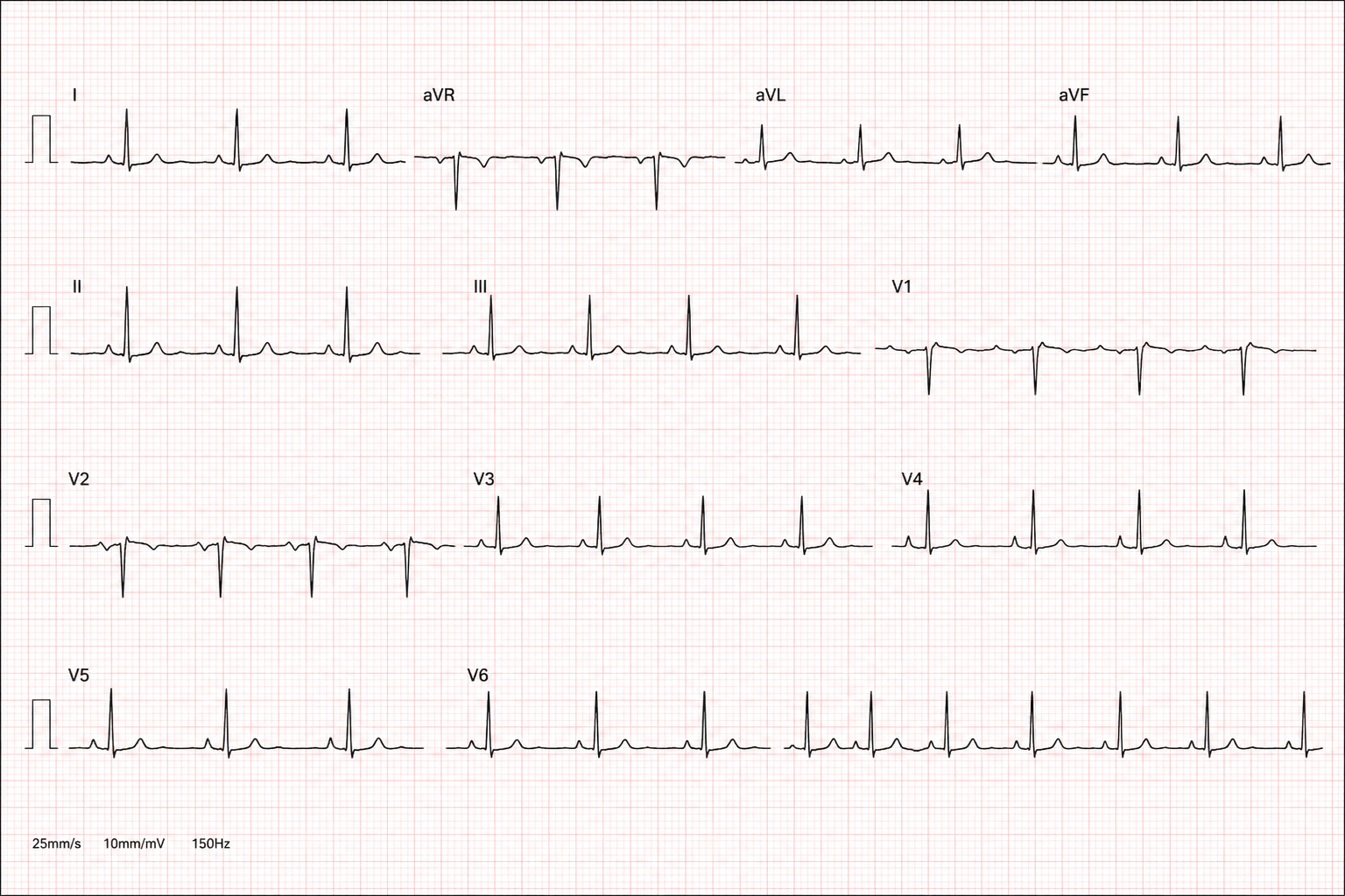
Representative 12-lead ECG
At first glance, ECG interpretation looks like a natural fit for modern VLMs (Vision Language Models).
An ECG is read visually. The standard clinical artifact is a printed plot: twelve traces in a 3×4 montage, laid over a millimetre grid, usually ten seconds wide. Cardiologists read shapes, intervals, slopes, axes, and relationships between leads. They are not looking at a raw digital sample buffer; they are reading a structured image.
That puts ECG diagnosis at exactly the level where frontier VLMs often look strong: pattern recognition over a structured image with a short, structured answer.
But ECG plots are also deeply out of distribution for general VLM pre-training. Web-scale image corpora contain photos, screenshots, charts, diagrams, and documents. They contain very few clinically meaningful 12-lead ECG plots, and almost no supervision about what P-wave morphology, ST-segment slope, QRS duration, or reciprocal changes mean.
The real question is whether it can extract clinically meaningful signal from the waveform image.
That is what we set out to measure.
The evaluation trap
ECG-VLM evaluation has three obvious traps.
The first is class imbalance. ECG datasets are not evenly distributed. Normal sinus rhythm is common. So are a handful of axis labels. A model can post respectable accuracy by predicting the most frequent answer again and again.
The second is measurement leakage. Many ECG prompts include machine-generated values such as heart rate, PR interval, QRS duration, QTc, and electrical axis. Those numbers are useful clinically, but they also create a shortcut. A model can infer some labels directly from the text without reading the waveform.
The third is sparse labeling. A single ECG can contain several findings, but the recorded diagnosis often includes only the most obvious one. A tracing might show a rhythm abnormality, a conduction defect, and ischemic changes, while the label names just one. Train on that target and the model learns to emit a single finding and leave the rest blank.
This is why aggregate accuracy is not enough.
A model can look like it is improving while relying on priors, leaked measurements, or incomplete labels. To evaluate waveform understanding, we needed to break performance down by diagnostic axis, compare every axis against its own majority-class baseline, and separate findings that can be inferred from the prompt from findings that require reading the trace.
What we tested
We used a curated dataset of real 12-lead ECG plots, on the order of one thousand examples. Each example contained:
a standard 12-lead ECG image,
machine-measured features such as heart rate, intervals, and axes,
a clinician diagnosis,
and a rationale explaining the diagnosis.
The labels covered everyday cardiology findings: sinus rhythms, conduction blocks, axis deviations, ischemic patterns, chamber abnormalities, and related ECG diagnoses.
The dataset had two properties that matter for evaluation.
First, the label space was fine-grained and long-tailed. A flat top-1 accuracy score is therefore treacherous: the modal prior is strong, and rare classes have too few examples to dominate the loss.
Second, the ground truth was often sparse. A tracing with rhythm, conduction, and ischemic findings might be recorded under only one salient diagnosis. That makes naive multi-label training unstable unless the target explicitly marks normal or absent findings on every axis.
We ran seven experiments to test where the model was getting stuck.
Experiment 1 — Zero-shot baselines
We first evaluated frontier APIs and small open VLMs zero-shot on the held-out ECG diagnosis task.
| Model | GPT-5.5 | Gemma-4B | Claude-Opus-4.7 | GPT-5.4 | Qwen3-VL-8B | Gemini-3.1-Flash-Lite |
|---|---|---|---|---|---|---|
| Top-1 accuracy | 32.5% | 31.4% | 24.5% | 22.7% | 16.6% | 13.0% |
Two things stood out.
First, the spread between models was much larger than we usually see on text-heavy benchmarks. ECG interpretation is off-distribution enough to expose meaningful differences in visual reasoning.
Second, even the strongest model was only modestly above trivial baselines. On the binary normal/abnormal version, frontier models cleared the always-abnormal baseline by only a few points. That is not enough margin for a product decision.
Zero-shot VLM ECG diagnosis was not reliable. The next question was whether supervised fine-tuning could close the gap.
Experiment 2 — Naive flat-label SFT
The simplest setup was image-to-label fine-tuning.
We trained Qwen3-VL-8B with LoRA adapters on ECG images paired with a single flat diagnosis string. No taxonomy. No per-axis decomposition. No explicit reasoning structure.
The result was effectively collapse.
Macro-F1 was 0.014. Almost every prediction collapsed onto two head labels: “left axis deviation” and “normal sinus rhythm.”
This did not tell us that the model could not see ECGs. It told us that a flat long-tailed label target was the wrong objective. With roughly one thousand images spread across many rare classes, the cheapest cross-entropy policy was to predict the head of the distribution and absorb the tail loss.
So we simplified the label space.
Experiment 3 — Binary normal/abnormal SFT
If the flat label space was too sparse, a binary target should help.
We fine-tuned Qwen3-VL-8B and Gemma-4B on normal versus abnormal classification.
The result was modest and did not generalize. On the held-out test split, the model failed to meaningfully clear the trivial always-abnormal baseline, which was about 74% on this set.
Binary classification made the failure less visible, but it did not solve it. If the model is not extracting waveform features, collapsing the label space only moves it closer to a trivial baseline.
That pushed us toward a structured benchmark.
Experiment 4 — Sparse taxonomy SFT
ECG diagnoses are compositional. “Old inferior MI with left axis deviation” is not one atomic class; it is a combination of findings.
So we rebuilt the target as an eight-axis taxonomy grounded in the AHA Diagnostic Statement List, the SCP-ECG standard, and PTB-XL superclasses. Instead of predicting one flat label, the model emitted a structured JSON object with one key per diagnostic axis.
This helped formatting, but not interpretation.
Both Qwen3-VL-8B and Gemma-4-E4B learned to emit valid JSON with zero parse failures. But they still populated only one axis per ECG on average, close to the sparse ground-truth pattern. Rare axes fired almost never.
The model had learned the schema, not the composition.
The sparse target was teaching it: “pick one salient finding and leave everything else empty.” That is not a useful benchmark for multi-finding ECG interpretation.
So we made every axis explicit.
Experiment 5 — Dense taxonomy SFT
We rewrote the target so every axis had a value, including explicit “normal” or “none” values for negative findings. We also consolidated rare findings and added a reasoning preamble before the final JSON.
A representative target looked like this:
{
"rate": "normal",
"rhythm": "sinus",
"axis": "left",
"conduction": "none",
"ischemia": {
"stage": "old",
"territory": "inferior"
},
"other_findings": [],
"diagnosis": "old inferior MI, left axis deviation"
}
This fixed the single-finding formatting collapse. It also revealed the deeper problem.
| Axis | Majority baseline | Qwen3-VL-8B dense | Gemma-4-E4B dense |
|---|---|---|---|
| Rate | 71.5% | 98.2% | 92.1% |
| Axis | 73.6% | 85.2% | 81.6% |
| Rhythm | 94.2% | 93.1% | 93.9% |
| Conduction | 80.9% | 79.8% | 80.5% |
| Ischemia stage | 70.0% | 60.7% | 70.0% |
| Diagnosis | — | 27.8% | 35.0% |
| Findings / ECG | GT ≈ 1.4 | 0.97 | 0.61 |
Rate and axis improved sharply. Rhythm, conduction, and ischemia did not.
That is the key diagnostic split. Heart rate and electrical axis were available in the machine-measurement text. Rhythm, conduction, and ischemia required visual waveform interpretation.
SFT worked when the relevant information was present in the prompt. It failed when the relevant information was only in the image.
At that point, the label target was no longer the obvious culprit. We turned to the image.
Experiment 6 — Image preprocessing
| Axis | Majority baseline | Dense baseline | Clean | Stacked |
|---|---|---|---|---|
| Rate | 71.5% | 92.1% | 92.8% | 94.6% |
| Axis | 73.6% | 81.6% | 80.5% | 81.6% |
| Rhythm | 94.2% | 93.9% | 94.2% | 94.2% |
| Conduction | 80.9% | 80.5% | 79.8% | 81.2% |
| Ischemia stage | 70.0% | 70.0% | 70.4% | 69.7% |
| Diagnosis | — | 35.0% | 32.5% | 31.8% |
The image-dependent axes did not move.
Rhythm stayed at the majority baseline. Ischemia stayed at the majority baseline. Conduction stayed within noise.
Grid removal and per-lead widening did not make the waveform usable to the model.
Maybe the model could not read the ECG because the image was visually hostile.
Two things seemed plausible:
the pink ECG grid added clutter,
Each lead was too small inside the standard 3×4 montage.
We built two preprocessed image variants.
Clean removed the grid using a chroma rule, then binarized and slightly dilated the waveform trace while preserving the original montage layout.
Stacked used the same grid removal but rearranged the twelve leads into full-width horizontal strips, giving each lead roughly four times more horizontal resolution.
We retrained Gemma-4-E4B on the dense task.
Experiment 7 — 12-lead patch multi-image input
The strongest version of the resolution hypothesis was to stop forcing all twelve leads through one image budget.
We split each ECG into twelve separate lead patches, removed the grid, upscaled each patch, and fed the model a twelve-image input in known lead order. Each lead now received its own image-token stream.
If the bottleneck was per-lead resolution or encoder budget, this should have helped.
It did not.
| Axis | Majority baseline | Dense baseline | 12-lead patch |
|---|---|---|---|
| Rate | 71.5% | 92.1% | 92.1% |
| Axis | 73.6% | 81.6% | 82.0% |
| Rhythm | 94.2% | 93.9% | 94.22% |
| Conduction | 80.9% | 80.5% | 81.6% |
| Ischemia stage | 70.0% | 70.0% | 70.04% |
| Diagnosis | — | 35.0% | 33.9% |
| Findings / ECG | GT ≈ 1.4 | 0.61 | 0.57 |
Rhythm landed on the majority class to two decimal places. Ischemia landed on the majority class to two decimal places. Conduction stayed within noise.
That gave us three independent negative image interventions:
remove visual clutter,
increase per-lead resolution,
increase per-lead encoder budget.
None moved the waveform-dependent axes off baseline.
Seven experiments, one result
Putting the per-axis experiments side by side makes the pattern clear.
| Axis | Maj. Baseline | Dense Gemma | Dense Qwen | Image-clean | Image-stacked | 12-lead patch |
|---|---|---|---|---|---|---|
| Rate | 71.5% | 92.1% | 98.2% | 92.8% | 94.6% | 92.1% |
| Axis | 73.6% | 81.6% | 85.2% | 80.5% | 81.6% | 82.0% |
| Rhythm | 94.2% | 93.9% | 93.1% | 94.2% | 94.2% | 94.2% |
| Conduction | 80.9% | 80.5% | 79.8% | 79.8% | 81.2% | 81.6% |
| Ischemia stage | 70.0% | 70.0% | 60.7% | 70.4% | 69.7% | 70.0% |
| Diagnosis | — | 35.0% | 27.8% | 32.5% | 31.8% | 33.9% |
| Findings / ECG | GT ≈ 1.4 | 0.61 | 0.97 | 0.62 | 0.61 | 0.57 |
Only two rows consistently clear baseline: rate and axis.
Those are the rows the model can infer from text measurements.
The waveform rows — rhythm, conduction, ischemia — do not improve across dense labels, sparse labels, grid removal, stacked leads, 12-lead patches, Qwen, or Gemma.
The model is not producing random errors. It is learning the prior.
That distinction matters. A wrong but varied model may be extracting some signal. A model that predicts the modal label on every example is telling you that the useful features are not available to the head, or that the dataset and objective do not make them learnable.
In our experiments, the same prior-aligned failure appeared across models, target formats, and image variants.
What we ruled out
This was not primarily an output-formatting problem. From the taxonomy experiments onward, the models emitted valid JSON reliably.
It was not simply a capacity problem. The same fine-tuning setup learned rate and axis well. Training loss decreased normally. LoRA SFT could move the model when the input contained a usable signal.
It was not fixed by obvious image preprocessing. Removing the grid, widening leads, and splitting leads into separate image inputs did not move rhythm, conduction, or ischemia off baseline.
The most likely explanation is an encoder-feature problem: general VLM image encoders are not organized around ECG morphology. The features a cardiologist uses — P-wave visibility, PR prolongation, QRS width, ST slope, T-wave morphology, reciprocal changes across leads — are extremely small, specialized visual signals. They are not the kind of features general web-image pretraining is optimized to preserve.
This is also why signal-native ECG foundation models are a different category. They pretrain on ECG signals directly, often at massive scale. A general VLM looking at a rendered ECG image starts from a very different prior.
Building a useful ECG-VLM benchmark
ECG AI can look convincing for the wrong reasons.
A model may learn shortcuts around the ECG without learning to interpret the waveform itself.
That is what we saw in our experiments. Supervised fine-tuning improved performance on findings that could be inferred from machine-generated measurements included in the prompt. It did not improve the findings that required reading the trace. Removing the grid, rearranging the leads, and feeding each lead as a separate image did not change the result.
This is why a single accuracy number is not enough.
A model can score reasonably well by predicting the most common label, using measurements already available in the prompt, or identifying one obvious abnormality while missing the rest of the ECG.
Our benchmark is designed to separate those cases. We report performance for each diagnostic axis and compare it against the majority-class baseline for that axis. We separate findings that can be inferred from text measurements from findings that require waveform interpretation. We also track how many findings the model reports per ECG, since a real trace often contains more than one abnormality.
Finally, we test whether the result changes across different image formats: the original ECG plot, a grid-removed version, stacked leads, and individual lead crops.
The question is not simply whether the model produced the right label.
It is how much of the diagnosis was actually supported by the trace.
That distinction matters before making a product bet. A model can look promising on aggregate accuracy and still fail on the findings that require genuine ECG interpretation.
That is the distinction we care about.
BioStack is building RL envs, evals, and datasets powering medical AI — sourced from real-world clinical settings.
If you are training, evaluating, or diligence-testing an ECG model, we can run it against this benchmark and tell you whether it is actually reading the ECG — or just exploiting priors, prompt leakage, and label imbalance.
Get in touch at sanat@getbiostack.com / parth@getbiostack.com